Python heapq module: Using heaps and priority queues

Table of contents

What are Heaps?
Heaps in the form of lists in the Python heapq module
- Basic operations
- High-level operation
Problems that Can Be Solved by a Bunch of People
How to identify problems
Example: Pathfinding
Conclusion

Heaps and priority queues are little-known but surprisingly useful data structures. They offer an easy-to-use and highly efficient solution for many tasks related to finding the best item in a dataset. The Python module heapq is part of the standard library. It implements all low-level heap operations, as well as some high-level common heap usage methods.

Priority Queue is a powerful tool that can solve tasks as diverse as scheduling emails, finding the shortest path on a map, or merging log files. Programming is full of optimization problems in which the goal is to find the best element. Priority queues and functions in the Python module heapq can often help with this.

In this lesson, you will learn:

What are heaps and priority queues and how are they related to each other
What problems can be solved with a bunch
How to use the Python module heapq to solve these problems

This guide is intended for those who understand Python and who are familiar with lists., dicts, sets, and generators and search for more complex data structures.

You can see the examples from this guide by downloading the source code from the link below:

Get the source code: Click here to get the source code that you will use to familiarize yourself with the Python heapq module in this tutorial.

What are Heaps?

Heaps are concrete data structures, while priority queues are abstract data structures. The abstract data structure defines the interface, while the concrete data structure defines the implementation.

Heaps are usually used to implement priority queues. They are the most popular concrete data structure for implementing an abstract priority queue data structure.

Specific data structures also define performance guarantees. Performance guarantees determine the ratio between the size of the structure and the time spent on performing operations. Understanding these guarantees allows you to predict how long it will take the program to resize the input data.

Data structures, heaps, and priority queues

Abstract data structures define operations and the relationships between them. For example, the abstract data structure of a priority queue supports three operations:

is_empty checks if the queue is empty.
add_element adds an item to the queue.
pop_element outputs the element with the highest priority.

Priority queues are usually used to optimize the execution of tasks that aim to complete the task with the highest priority. After the task is completed, its priority is reduced and it is returned to the queue.

There are two different conventions for determining the priority of an element:

The largest element has the highest priority.
The smallest element has the highest priority .

These two conventions are equivalent because you can always change the order of the elements. For example, if your elements consist of numbers, then using negative numbers will change these conventions.

The Python module heapq uses the second convention, which is usually the more common of the two. According to this convention, the smallest element has the highest priority . This may seem unexpected, but it is often very useful. In the real-world examples that you'll see later, this convention will simplify your code.

Note: The Python module heapq and the heap data structure as a whole are not designed to allow you to find any element except the smallest. To search for any element by size, the best option is a binary search tree.

Specific data structures implement the operations defined in the abstract data structure and additionally define performance guarantees.

The implementation of a priority queue in the heap ensures that both moving (adding) and deleting (popping) items are performed in logarithmic time operations. This means that the time required to perform push and pop operations is proportional to the logarithm base 2 of the number of elements.

Logarithms grow slowly. The logarithm of the number fifteen in base 2 is about four, while the logarithm of a trillion in base 2 is about forty. This means that if an algorithm is fast enough on fifteen elements, then it will run only ten times slower on a trillion elements and will probably still be fast enough.

In any discussion of performance, the biggest caveat is that these abstract considerations are less important than actually measuring a specific program and examining where the bottlenecks are. General performance guarantees are still important for making useful predictions about program behavior, but these predictions must be validated.

Heap implementation

The heap implements a priority queue in the form of a complete binary tree. In a binary tree, each node will have at most two child nodes. In a complete binary tree, all levels, with the possible exception of the deepest, are always filled. If the deepest level is not completed, then its vertices will be located as far to the left as possible.

The completeness property means that the depth of the tree is equal to the logarithm of the number of elements in base 2, rounded up. Here is an example of a complete binary tree:

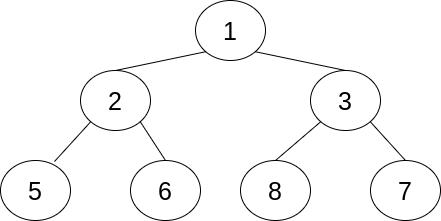
In this particular example, all levels are completed. Each node, except for the deepest ones, has exactly two child nodes. There are seven nodes on three levels in total. Three is the logarithm of the number seven in base 2, rounded up.

The only node at the basic level is called the root node. It may seem strange to call a node at the top of the tree the root node, but this is a common practice in programming and computer science.

The performance guarantees on the heap depend on how the elements move up and down the tree. The practical result of this is that the number of comparisons in the heap is equal to the logarithm of the base 2 tree size.

Note: Comparisons sometimes involve invoking custom code using .__lt__(). Calling custom methods in Python is a relatively slow operation compared to other operations performed on the heap, so it is usually a bottleneck.

In the heap tree, the value in a node is always less than that of both of its children. This is called the heap property. This differs from the binary search tree, in which only the left node will be less than the value of its parent element.

The algorithms for both moving and popping are based on temporarily violating the heap property, and then correcting the heap property through comparisons and substitutions up or down one branch.

For example, to put an item on the heap, Python adds a new node to the next open slot. If the bottom layer is not filled, then the node is added to the next open slot at the bottom. Otherwise, a new layer is created, and then the element is added to a new lower layer.

As soon as a node is added, Python compares it with the parent node. If the heap property is violated, then the node and its parent element are swapped, and the check starts again from the parent element. This continues until the heap property is satisfied or the root is reached.

Similarly, when displaying the smallest element, Python knows that due to the heap property, this element is located at the root of the tree. It replaces the element with the last element at the deepest level, and then checks if the heap property is broken further down the branch.

Using priority queues

The priority queue and the heap as its implementation are useful for programs that require searching for an element that is extreme in some way. For example, you can use a priority queue for any of the following tasks:

Getting the three most popular blog entries based on traffic data
Finding the fastest way to get from one point to another
Predicting which bus will arrive at the station first based on arrival frequency

Another task that you could use a priority queue for is email scheduling. Imagine a system in which there are several types of emails, each of which must be sent with a certain frequency. One email should be sent every fifteen minutes and another every forty minutes.

The scheduler can add both types of emails to the queue with a timestamp indicating when the email should be sent next. The scheduler could then look at the item with the smallest timestamp indicating that it is next in line to be shipped, and calculate how long to wait before shipping.

When the scheduler wakes up, it will process the corresponding email, remove it from the priority queue, calculate the next timestamp, and return the email to the queue at the appropriate location.

Heaps in the form of lists in the Python module `heapq`

Although you have seen the heap described earlier in the form of a tree, it is important to remember that this is a complete binary tree. Completeness means that it is always possible to determine how many elements are on each level, except for the last one. Due to this, heaps can be implemented as a list. This is what the Python module does. heapq.

There are three rules that define the relationship between an element with an index k and its surrounding elements.:

Its first child element is in 2*k + 1.
Its second child element is located at 2*k + 2.
Its parent element is located at (k - 1) // 2.

Note: The // symbol is the integer division operator. It always rounds the value down to an integer.

The rules above explain how to visualize a list as a complete binary tree. Keep in mind that an element always has a parent element, but some elements do not have child elements. If 2*k is outside the end of the list, then the element has no child elements. If 2*k + 1 is a valid index, but 2*k + 2 is not, then the element has only one child element.

The heap property means that if h is a heap, then the following will never happen False:

h[k] <= h[2*k + 1] and h[k] <= h[2*k + 2]

This can lead to IndexError if any of the indexes exceed the length of the list, but this will never happen. False.

In other words, an element must always be smaller than elements that have twice its index plus one and twice its index plus two.

Here is a visual image of a list that satisfies the heap property:

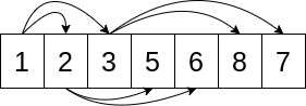
The arrows lead from the k element to the 2*k + 1 and 2*k + 2 elements. For example, the first element in the Python list has an index 0, so its two arrows point to the indexes 1 and 2. Note that the arrows always go from a lower value to a higher value. Here's how you can check if the list satisfies the heap property.

Basic operations

The Python module heapq implements operations with a bunch of lists. Unlike many other modules, it does not define a custom class. The Python module heapq has functions that work directly with lists.

Usually, as in the email example above, the items will be inserted into the pile one by one, starting from an empty pile. However, if there is already a list of items that should be represented as a heap, then the Python module heapq includes heapify() to convert the list into a valid heap.

The following code uses heapify() to convert a into a heap :

>>> import heapq
>>> a = [3, 5, 1, 2, 6, 8, 7]
>>> heapq.heapify(a)
>>> a
[1, 2, 3, 5, 6, 8, 7]

You can check that although 7 follows 8, the list a still obeys the heap property. For example, a[2], which is 3, is less than a[2*2 + 2], which is 7.

As you can see, heapify() changes the list in place, but does not sort it. The heap does not have to be sorted to satisfy the heap property. However, since each sorted list satisfies the heap property, doing heapify() for the sorted list will not change the order of the elements in the list.

Other basic operations in the Python module heapq assume that the list is already a heap. It is useful to note that an empty list or a list with a length of one will always be a heap.

Since the root of the tree is the first element, you don't need a special function to non-destructively read the smallest element. The first element, a[0], will always be the smallest element.

To extract the smallest element while preserving the heap property, the Python module heapq defines heappop().

Here's how to use heappop() to display an element:

>>> import heapq
>>> a = [1, 2, 3, 5, 6, 8, 7]
>>> heapq.heappop(a)
1
>>> a
[2, 5, 3, 7, 6, 8]

The function returns the first element, 1, and stores the heap property for a. For example, a[1] is 5, and a[1*2 + 2] is 6.

The Python module heapq also includes heappush() for moving an item to a heap while preserving the heap property.

The following example shows moving a value to a heap:

>>> import heapq
>>> a = [2, 5, 3, 7, 6, 8]
>>> heapq.heappush(a, 4)
>>> a
[2, 5, 3, 7, 6, 8, 4]
>>> heapq.heappop(a)
2
>>> heapq.heappop(a)
3
>>> heapq.heappop(a)
4

After moving 4 to the pile, you extract three items from it. Since 2 and 3 were already in the heap and are smaller than 4, they are extracted first.

The Python module heapq also defines two more operations:

heapreplace() equivalent to heappop(), followed by heappush().
heappushpop() equivalent to heappush(), followed by heappop().

This is useful in some algorithms because they are more efficient than performing two operations separately.

High-level operation

Because priority queues are so often used to combine sorted sequences, the Python module heapq has a ready-made function merge() to use heaps to combine multiple iterations. merge() assumes that its input iterative values are already sorted and returns an iterator , not a list.

As an example of using merge(), here is the implementation of the email scheduler described earlier:

import datetime
import heapq

def email(frequency, details):
    current = datetime.datetime.now()
    while True:
        current += frequency
        yield current, details

fast_email = email(datetime.timedelta(minutes=15), "fast email")
slow_email = email(datetime.timedelta(minutes=40), "slow email")

unified = heapq.merge(fast_email, slow_email)

The input data for merge() in this example are infinite generators. The return value assigned to the unified variable is also an infinite iterator. This iterator will output emails that will be sent in the order of future timestamps.

To debug and confirm the correctness of combining the code, you can print the first ten emails to send:

>>> for _ in range(10):
...    print(next(element))
(datetime.datetime(2020, 4, 12, 21, 27, 20, 305358), 'fast email')
(datetime.datetime(2020, 4, 12, 21, 42, 20, 305358), 'fast email')
(datetime.datetime(2020, 4, 12, 21, 52, 20, 305360), 'slow email')
(datetime.datetime(2020, 4, 12, 21, 57, 20, 305358), 'fast email')
(datetime.datetime(2020, 4, 12, 22, 12, 20, 305358), 'fast email')
(datetime.datetime(2020, 4, 12, 22, 27, 20, 305358), 'fast email')
(datetime.datetime(2020, 4, 12, 22, 32, 20, 305360), 'slow email')
(datetime.datetime(2020, 4, 12, 22, 42, 20, 305358), 'fast email')
(datetime.datetime(2020, 4, 12, 22, 57, 20, 305358), 'fast email')
(datetime.datetime(2020, 4, 12, 23, 12, 20, 305358), 'fast email')

Please note that fast email is assigned every 15 minutes, slow email is assigned every 40, and the emails are correctly interleaved so that they are arranged in a certain order. the order of their timestamps.

merge() It does not read the entire input, but works dynamically. Even though both inputs are infinite iterators, printing the first ten elements is fast.

Similarly, when combining sorted sequences such as log file lines ordered by timestamps, even if the logs are large, it will take a reasonable amount of memory.

Heaps of problems can be solved

As you saw above, heaps are good for gradually combining sorted sequences. The two heap applications you've already considered are scheduling periodic tasks and merging log files. However, there are many more applications.

Heaps can also help identify the upper n or lower n objects. The Python module heapq has high-level functions that implement this behavior.

For example, this code takes as input the results of the women's 100-meter final at the 2016 Summer Olympics and outputs the medalists or the top three finishers:

>>> import heapq
>>> results="""\
... Christania Williams      11.80
... Marie-Josee Ta Lou       10.86
... Elaine Thompson          10.71
... Tori Bowie               10.83
... Shelly-Ann Fraser-Pryce  10.86
... English Gardner          10.94
... Michelle-Lee Ahye        10.92
... Dafne Schippers          10.90
... """
>>> top_3 = heapq.nsmallest(
...     3, results.splitlines(), key=lambda x: float(x.split()[-1])
... )
>>> print("\n".join(top_3))
Elaine Thompson          10.71
Tori Bowie               10.83
Marie-Josee Ta Lou       10.86

This code uses nsmallest() from the Python module heapq. nsmallest() returns the smallest elements in iterable and takes three arguments:

n specifies how many items to return.
iterable defines the elements or data set to be compared.
key this is a callable function that defines a way to compare elements.

Here, the function keysplits the string into spaces, takes the last element and converts it to a floating point number. This means that the code will sort the rows by execution time and return the three rows with the shortest execution time. They correspond to the three fastest runners, which allows you to get gold, silver and bronze medals.

The Python module heapq also includes nlargest(), which has similar parameters and returns the largest elements. This would be useful if you would like to receive the winners of the javelin throwing competitions, the purpose of which is to throw the javelin as far as possible.

How to identify problems

A heap, as an implementation of a priority queue, is a good tool for solving problems related to extreme values, such as the largest or smallest value of a given metric.

There are other words that indicate that a bunch can be useful:

The biggest
The smallest
Big
Small
The best
The worst
Upper
Nizhny
Maximum
Minimum
Optimal

Whenever the problem statement indicates that you are looking for some extreme element, it is worth considering whether a priority queue would be useful.

Sometimes the priority queue will be only part of the solution, and the rest will be some variant of dynamic programming. This is exactly the case with the full example, which you will see in the next section. Dynamic programming and priority queues are often useful together.

Example: Pathfinding

The following example is a realistic example of using a Python module heapq. The example will use a classical algorithm, which, as one of its parts, requires the use of a heap. You can download the source code used in the examples by clicking on the link below:

Get the source code: Click here to get the source code that you will use to familiarize yourself with the Python heapq module in this tutorial.

Imagine a robot that needs to navigate through a two-dimensional maze. The robot needs to walk from the origin, located in the upper-left corner, to the destination, located in the lower-right corner. A map of the maze is stored in the robot's memory, so it can plan the entire path before setting off.

The goal is for the robot to complete the maze as quickly as possible.

Our algorithm is a variant of the Dijkstra algorithm. There are three data structures that are saved and updated throughout the algorithm.:

tentative This is a map of the approximate path from the origin to a certain position, pos. This path is called preliminary because it is the shortest of the known paths, but it can be improved.
certain this is a set of points for which the path displayed on tentative is defined and is the shortest possible path.
candidates this is a bunch of positions that have a path. The sorting key of the heap is the length of the path.

You can perform up to four actions at each step.:

Select a candidate from candidates.
Add the candidate to the set certain. If the candidate is already a member of the certain set, skip the following two steps.
Find the shortest known path to the current candidate.
For each of the current candidate's nearest neighbors, see if passing through the candidate gives a path shorter than the current path tentative. If so, update the tentative path and the candidates heap with this new path.

The steps are performed in a loop until the destination is added to the set certain. When the destination is in the set certain, everything is ready. The result of the algorithm is tentative the path to the destination, which is now certain the shortest possible path.

Top-level code

Now that you have understood the algorithm, it's time to write the code to implement it. Before implementing the algorithm itself, it is useful to write some auxiliary code.

First you need to import the Python module heapq:

import heapq

You will use functions from the Python module heapq to support the heap, which will help you find the position with the shortest known path at each iteration.

The next step is to define the map as a variable in the code:

map = """\
.......X..
.......X..
....XXXX..
..........
..........
"""

The map is a string enclosed in triple quotes, which shows the area where the robot can move, as well as any obstacles.

Although in a more realistic scenario you would be reading a map from a file, for educational purposes it is easier to define a variable in the code using this simple map. The code will work on any map, but it is easier to understand and debug on a simple map.

This map is optimized in such a way that it is easy for the user reading the code to understand. The dot (.) is light enough to look empty, but it has the advantage of showing the size of the allowed area. The positions X indicate obstacles that the robot cannot overcome.

Support code

The first function transforms the map into something easier to analyze in code. parse_map() receives the map and analyzes it:

def parse_map(map):
    lines = map.splitlines()
    origin = 0, 0
    destination = len(lines[-1]) - 1, len(lines) - 1
    return lines, origin, destination

The function takes a map and returns a tuple of three elements:

The list lines
The most origin
In destination

This allows the rest of the code to work with data structures designed for computers, rather than for visual scanning by humans.

The list lines can be indexed by coordinates (x, y). The expression lines[y][x] returns the position value as one of two characters:

Period (".") indicates that the position is an empty space.
The letter "X" indicates that this position is an obstacle.

This will be useful if you want to determine which positions a robot can occupy.

The is_valid() function calculates whether a given position (x, y) is valid:

def is_valid(lines, position):
    x, y = position
    if not (0 <= y < len(lines) and 0 <= x < len(lines[y])):
        return False
    if lines[y][x] == "X":
        return False
    return True

This function takes two arguments:

lines It is a map in the form of a list of lines.
position this is the position to check in the form of two sets of integers indicating the coordinates. (x, y).

For a position to be valid, it must be located within the boundaries of the map and not be an obstacle.

The function checks the validity of y by checking the length of the list lines. The function then checks that x is valid, making sure that it is inside lines[y]. Finally, now that you know that both coordinates are inside the map, the code verifies that they are not an obstacle by looking at the symbol at that position and comparing it with "X".

Another useful helper is get_neighbors(), which finds all the neighbors of a position.:

def get_neighbors(lines, current):
    x, y = current
    for dx in [-1, 0, 1]:
        for dy in [-1, 0, 1]:
            if dx == 0 and dy == 0:
                continue
            position = x + dx, y + dy
            if is_valid(lines, position):
                yield position

The function returns all valid positions surrounding the current position.

get_neighbors() It tries to avoid identifying a position as its own neighbor, but allows for diagonal neighbors. That's why at least one of dx and dy should not be zero, but it's quite normal that both of them are not zero.

The last auxiliary function is get_shorter_paths(), which finds shorter paths:

def get_shorter_paths(tentative, positions, through):
    path = tentative[through] + [through]
    for position in positions:
        if position in tentative and len(tentative[position]) <= len(path):
            continue
        yield position, path

get_shorter_paths() returns positions for which the path having through as the last step is shorter than the current known path.

get_shorter_paths() it has three parameters:

tentative This is a dictionary that displays the location along the shortest known path.
positions this is a repeating set of positions that you want to shorten the path to.
through this is a position through which, perhaps, a shorter path can be found to positions.

It is assumed that all the elements in positions can be accessed in one step from through.

The get_shorter_paths() function checks whether using through as the last step will create the best path for each position. If the path to the position is unknown, then any path is shorter. If there is a known path, then the new path will only be available if its length is shorter. To simplify the use of the get_shorter_paths() API, the yield part is also a shorter path.

All the auxiliary functions were written as pure functions, which means that they do not change any data structures and return only values. This makes it easier to use the main algorithm that performs all updates to the data structure.

The code of the main algorithm

So, you're looking for the shortest path between your starting point and your destination.

You are saving three pieces of data:

certain this is a set of specific positions.
candidates There are a lot of candidates.
tentative It is a dictionary that maps nodes to the current shortest known path.

The position is at certain if you can be sure that the shortest known path is the shortest possible path. If the destination is specified in certain, then the shortest known path to the destination is undoubtedly the shortest possible path, and you can return along this path.

The heap candidates is organized by the length of the shortest known path and is controlled using functions in the Python module heapq.

At each step, you look at the candidate with the shortest known path. This is where heappop() appears in the pile. There is no shorter path to this candidate — all other paths pass through some other node in candidates, and they are all longer. Because of this, the current candidate may be marked certain.

Then you look through all the neighbors that have not been visited, and if traversing the current node is an improvement, then you add them to the pile candidates using heappush().

The find_path() function implements this algorithm:

 1def find_path(map):
 2    lines, origin, destination = parse_map(map)
 3    tentative = {origin: []}
 4    candidates = [(0, origin)]
 5    certain = set()
 6    while destination not in certain and len(candidates) > 0:
 7        _ignored, current = heapq.heappop(candidates)
 8        if current in certain:
 9            continue
10        certain.add(current)
11        neighbors = set(get_neighbors(lines, current)) - certain
12        shorter = get_shorter_paths(tentative, neighbors, current)
13        for neighbor, path in shorter:
14            tentative[neighbor] = path
15            heapq.heappush(candidates, (len(path), neighbor))
16    if destination in tentative:
17        return tentative[destination] + [destination]
18    else:
19        raise ValueError("no path")

find_path() gets map as a string and returns the path from the source to the destination as a list of positions.

This function is a bit long and complicated, so let's look at it in order:

Lines 2 to 5 specify the variables that the loop will view and update. You already know the path from the origin to yourself, which is an empty path with length 0.
Line 6 defines the loop termination condition. If not candidates, then no paths can be shortened. If destination is located in certain, then the path to destination cannot be shortened.
Lines 7 through 10 get a candidate using heappop(), skip the loop if it already exists in certain, and otherwise add the candidate to certain. This ensures that each candidate will be processed by the loop no more than once.
In lines 11 to 15, get_neighbors() and get_shorter_paths() are used to find shorter paths to neighboring positions and update the dictionary tentative and candidates bunch.
Lines 16 to 19 return the correct result. If the path was found, the function returns it. Despite the fact that calculating paths without the end position simplified the implementation of the algorithm, it is more convenient for the API to return it with the addressee. If the path is not found, an exception occurs.

Breaking down a function into separate sections allows you to understand it in parts.

Visualization code

If the algorithm were actually used by a robot, then the robot would probably work better with a list of positions it has to traverse. However, to make the result more attractive to people, it would be more pleasant to visualize it.

show_path() draws a path on the map:

def show_path(path, map):
    lines = map.splitlines()
    for x, y in path:
        lines[y] = lines[y][:x] + "@" + lines[y][x + 1 :]
    return "\n".join(lines) + "\n"

The function takes the values path and map as parameters. It returns a new map with the route indicated by the symbol at ("@").

Running the code

Finally, you need to call the functions. This can be done using the interactive Python interpreter..

The following code will run the algorithm and show a beautiful result:

>>> path = find_path(map)
>>> print(show_path(path, map))
@@.....X..
..@....X..
...@XXXX..
....@@@@@.
.........@

First you get the shortest path from find_path(). Then you pass it to show_path() to display the map with the path marked on it. Finally, you print() convert the card to standard output.

The track moves one step to the right, then a few steps diagonally to the lower-right corner, then a few more steps to the right, and finally ends with a step diagonally to the lower-right corner.

Congratulations! You solved the problem using the Python module. heapq.

These kinds of pathfinding tasks, solved using a combination of dynamic programming and priority queues, are often found at job interviews and in programming tasks. For example, the appearance of the code in 2019 included a problem that could be solved using the methods described here.

Conclusion

Now you know what data structures heap and priority queue are and what tasks they are useful for. You have learned how to use the Python module heapq to use Python lists as heaps. You also learned how to use high-level operations in the Python module heapq, such as merge(), which internally use the heap.

In this guide, you've learned how to:

Use low-level functions in the Python module heapq to solve problems that require a heap or a priority queue
Use high-level functions in the Python module heapq to combine sorted iterations or search for the largest or smallest elements in the iteration table
Recognize problems that can help solve heaps and priority queues
Predict performance code using heaps