Combining data in pandas using the merge(), .join(), and concat() functions
Table of contents
- pandas merge(): Combining data by common columns or indexes.
- pandas .join(): Joins data in a column or index.
- pandas concat(): Combining data in rows or columns.
- Conclusion
Objects Series and DataFrame in pandas are powerful tools for studying and analyzing data. Some of their capabilities are due to a multi-faceted approach to combining individual data sets. With pandas, you can combine, combine and combine your datasets, which allows you to unify and understand your data better as you analyze it.
In this guide, you will learn how and when to combine your data in pandas with:
merge()to combine data by common columns or indexes.join()to combine data into a key column or indexconcat()to combine data frames by rows or columns
If you have some experience using objects DataFrame and Series in pandas and you are ready to learn how to combine them, then this guide will help you do just that. If you're feeling a little tired, you can watch a brief overview of data frameworks before continuing.
You can read the examples from this guide using Jupyter interactive Notepad and the data files available at the link below:
Download the notebook and data set: Click here to get the Jupyter notebook and the CSV dataset that you will use to familiarize yourself with Pandas, this guide uses the merge(), .join() and concat functions.().
Note: The methods that you will learn about below will usually work with both DataFrame and Series objects. But for simplicity and brevity, the examples will use the term dataset to refer to objects that can be either data frames or series.
pandas merge(): Combining data by common columns or indexes
The first technique you will learn is merge(). You can use merge() anytime you need functionality similar to database pooling operations in . This is the most flexible of the three operations that you will learn.
If you want to combine data objects based on one or more keys, similar to what you would do in a relational database, merge() is the tool you need. More specifically, merge() is most useful when you want to combine rows with common data.
You can perform both many-to-one and many-to-many connections with merge(). When combining many-to-one, there will be many rows in the join column of one of the datasets that repeat the same values. For example, the values can be 1, 1, 3, 5, and 5. At the same time, the join column in the other dataset will not have duplicate values. Let's take the values 1, 3, and 5 as an example.
As you might have guessed, with a many-to-many merge, both of your merge columns will have duplicate values. These merges are more complex and lead to the Cartesian product of the combined strings.
This means that after merging, you will have all the row combinations that have the same value in the key column. You will see this in action in the examples below.
What makes merge() so flexible is the huge number of options for defining the behavior of your merge. Although this list may seem intimidating, with practice you will be able to skillfully combine datasets of all kinds.
When you use merge(), you specify two required arguments:
- Data frame
left - The data frame
right
After that, you can specify a number of optional arguments that define how to combine your datasets:
-
howdetermines which type of merge should be performed. The default value is'inner', but other options are possible, including'outer','left', and'right'. -
onspecifiesmerge()to which columns or indexes, also called key columns or key indexes, you want to join. This is optional. If this is not specified, andleft_indexandright_index(described below) areFalse, then columns from two data frames that have common names will be used as join keys. If you useon, then the column or index you specified must be present in both objects. -
left_onandright_onspecify a column or index that is present only in the object.leftorright, which you combine. Both default values are equalNone. -
left_indexandright_indexboth default values areFalse, but if you want to use the index of the left or right joined object, then you can set the corresponding argument valueTrue. -
suffixesIt is a set of rows to add to identical column names that are not merge keys. This allows you to track the origin of columns with the same name.
These are some of the most important parameters that need to be passed to merge(). The full list is given in the documentation for pandas.
Note: In this guide, you will see that the examples always use on to specify which columns to join. This is the safest way to combine your data, because you and everyone who reads your code will know exactly what to expect when calling merge(). If you do not specify the columns to combine using on, then pandas will use any columns with the same name as the keys to combine.
How to use merge()
Before going into the details of using merge(), you should first understand the different forms of compounds:
innerouterleftright
Note: Even if you find out about the merger, you will see that inner, outer, left, and right are also called join operations. In this guide, you can consider the terms merge and merge equivalent.
You will learn more about these various connections below, but first take a look at their visual representation:
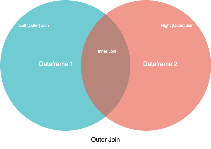 Visual representation of connection types
In this image, the two circles are your two datasets, and the labels indicate which part or portions of the datasets you expect to see. Although this diagram does not reveal all the nuances, it can be a convenient guide for those who study visual art.
If you have experience with SQL, then you can recognize the names of merge operations from the syntax JOIN. With the exception of inner, all these methods are types of external joins. Using external joins, you will combine your data based on all the keys in the left object, the right object, or both. For keys that exist only in one object, mismatched columns in another object will be filled in NaN, which means , not a number..
You can also find a visual explanation of the various joins in the context of SQL on the Coding Horror page. Now take a look at the various associations in action.
Examples
Many pandas manuals provide very simple data frames illustrating the concepts they are trying to explain. This approach can lead to confusion because you won't be able to link the data to anything specific. So, in this guide, you will use two real datasets as frameworks to combine:
- Climate standards for California (temperature)
- Climate standards for California (precipitation)
You can study these datasets and follow the examples below using Jupyter interactive notepad and CSV files of climate data:
Download the notebook and data set: Click here to get the Jupyter notebook and the CSV dataset that you will use to familiarize yourself with Pandas, this guide uses the merge(), .join() and concat functions.().
If you want to learn how to use Jupyter notebooks, check out Jupyter Notebook: Introduction.
These two datasets belong to the National Oceanic and Atmospheric Administration (NOAA) and were obtained from the NOAA public data repository. First, load the datasets into separate data frames:
>>> import pandas as pd
>>> climate_temp = pd.read_csv("climate_temp.csv")
>>> climate_precip = pd.read_csv("climate_precip.csv")
In the above code, you used pandas’ read_csv() for easy loading of the source CSV files into objects DataFrame. Then you can view the headers and the first few lines of the uploaded data frames using .head():
>>> climate_temp.head()
             STATION            STATION_NAME  ... DLY-HTDD-BASE60 DLY-HTDD-NORMAL
0  GHCND:USC00049099  TWENTYNINE PALMS CA US  ...              10              15
1  GHCND:USC00049099  TWENTYNINE PALMS CA US  ...              10              15
2  GHCND:USC00049099  TWENTYNINE PALMS CA US  ...              10              15
3  GHCND:USC00049099  TWENTYNINE PALMS CA US  ...              10              15
4  GHCND:USC00049099  TWENTYNINE PALMS CA US  ...              10              15

>>> climate_precip.head()
             STATION  ... DLY-SNOW-PCTALL-GE050TI
0  GHCND:USC00049099  ...                   -9999
1  GHCND:USC00049099  ...                   -9999
2  GHCND:USC00049099  ...                   -9999
3  GHCND:USC00049099  ...                       0
4  GHCND:USC00049099  ...                       0
Here you used .head() to get the first five rows of each data frame. Be sure to try it yourself, either using the Jupyter Notebook interactive notebook or using the console so that you can explore the data in more detail.
Next, take a look at the sizes of the two data frames:
>>> climate_temp.shape
(127020, 21)
>>> climate_precip.shape
(151110, 29)
Please note that .shape - this is a property of DataFrame objects that tells you the dimensions of the data frame. For climate_temp, the output .shape indicates that the data frame contains 127,020 rows and 21 columns.
Internal connection
In this example, you will use merge() with default arguments, which will result in an internal connection. Keep in mind that when merging internally, you will lose rows that do not match in the key column of another data frame.
After loading two datasets into objects DataFrame, you will select a small fragment of the precipitation dataset, and then use a simple call merge() to perform an internal merge. The result is a smaller and more focused dataset:
>>> precip_one_station = climate_precip.query("STATION == 'GHCND:USC00045721'")
>>> precip_one_station.head()
                STATION  ... DLY-SNOW-PCTALL-GE050TI
1460  GHCND:USC00045721  ...                   -9999
1461  GHCND:USC00045721  ...                   -9999
1462  GHCND:USC00045721  ...                   -9999
1463  GHCND:USC00045721  ...                   -9999
1464  GHCND:USC00045721  ...                   -9999
Here you have created a new data frame named precip_one_station from the data frame climate_precip, selecting only those rows in which the field STATION "GHCND:USC00045721".
If you check the shape attribute, you will see that it contains 365 lines. How many rows do you think will be in the combined data frame when you do the merge? Remember that you will be performing an internal connection:
>>> inner_merged = pd.merge(precip_one_station, climate_temp)
>>> inner_merged.head()
             STATION            STATION_NAME  ...  DLY-HTDD-BASE60  DLY-HTDD-NORMAL
0  GHCND:USC00045721  MITCHELL CAVERNS CA US  ...               14               19
1  GHCND:USC00045721  MITCHELL CAVERNS CA US  ...               14               19
2  GHCND:USC00045721  MITCHELL CAVERNS CA US  ...               14               19
3  GHCND:USC00045721  MITCHELL CAVERNS CA US  ...               14               19
4  GHCND:USC00045721  MITCHELL CAVERNS CA US  ...               14               19

>>> inner_merged.shape
(365, 47)
If you guessed right with 365 lines, then you were right! This is because merge() by default, an internal join is used, and with an internal join, only those lines that do not match are discarded. Since all your strings matched, none of them were lost. You should also notice that there are a lot more columns now: 47, to be exact.
You can also use merge() to control which columns to join. Let's say you want to combine both complete data sets, but only for Station and Date, because their combination will give a unique value for each row. To do this, you can use the parameter on:
>>> inner_merged_total = pd.merge(
...     climate_temp, climate_precip, on=["STATION", "DATE"]
... )
>>> inner_merged_total.shape
(123005, 48)
You can specify one key column with a row or several key columns with a list. The result is a data frame with 123,005 rows and 48 columns.
Why are there 48 columns instead of 47? Since you have specified the key columns to merge, pandas does not attempt to merge all the columns available for merging. This can lead to “duplicate” column names, which may or may not have different meanings.
“Duplicate” is enclosed in quotation marks because the column names will not match exactly. By default, _x and _y are added to them. You can also use the suffixes parameter to control what is added to the column names.
To avoid surprises, all of the following examples will use the on parameter to specify the column or columns to join.
External connection
Here you will specify an external connection with the how parameter. Remember from the diagrams above that with an external connection, also known as full external connection, all rows from both data frameworks will be present in the new data frame.
If a row does not match in another data frame based on key columns, then you will not lose the row as you would with an internal join. Instead, the row will be in a combined data frame, where values will be filled in if necessary. NaN.
This is best illustrated by an example:
>>> outer_merged = pd.merge(
...     precip_one_station, climate_temp, how="outer", on=["STATION", "DATE"]
... )
>>> outer_merged.shape
(127020, 48)
If you remember that you checked the .shape attribute in climate_temp, then you will see that the number of rows in outer_merged is the same. With an external connection, you can expect that the number of rows in it will be the same as in a larger data frame. This is because during an external connection, not a single row is lost, even if they do not match in another data frame.
Connection on the left
In this example, you will specify the left connection, also known as left external connection with the how parameter. Using an external connection on the left will cause all rows from the left data frame to remain in your new combined data frame, while at the same time removing rows from the right data frame that do not match in the key column of the left data frame.
You can think of it as a half-external, half-internal merge. The example below shows this in action.:
>>> left_merged = pd.merge(
...     climate_temp, precip_one_station, how="left", on=["STATION", "DATE"]
... )
>>> left_merged.shape
(127020, 48)
left_merged it contains 127,020 rows, which corresponds to the number of rows in the left data frame, climate_temp. To prove that this is true only for the left data frame, run the same code, but change the position precip_one_station and climate_temp:
>>> left_merged_reversed = pd.merge(
...     precip_one_station, climate_temp, how="left", on=["STATION", "DATE"]
... )
>>> left_merged_reversed.shape
(365, 48)
The result is a data frame with 365 rows, which corresponds to the number of rows in precip_one_station.
Correct connection
The right connection, or right external connection, is a mirror version of the left connection. With this combination, all rows from the right data frame will be saved, while rows in the left data frame that do not match in the key column of the right data frame will be discarded.
To demonstrate how the right and left connections mirror each other, in the example below you will recreate the left_merged Data frame from above, only this time using the right connection:
>>> right_merged = pd.merge(
...     precip_one_station, climate_temp, how="right", on=["STATION", "DATE"]
... )
>>> right_merged.shape
(127020, 48)
Here you just swapped the input data frames and specified the correct connection. When checking right_merged, you may notice that this is not exactly the same as left_merged. The only difference between them is the order of the columns: the columns of the first input will always be the first in the newly formed data frame.
merge() This is the most complex of the pandas data pooling tools. It is also the foundation upon which other tools are built. Its complexity is its greatest strength, allowing you to combine datasets in any way and gain new insights into your data.
On the other hand, this complexity makes it difficult to use merge() without an intuitive understanding of set theory and database operations. In this section, you will learn about various methods of combining data, as well as many-to-one and many-to-many merges, which are ultimately based on set theory. For more information about set theory, check out Sets in Python.
Now look at .join(), a simplified version merge().
pandas .join(): Combining data in a column or index
, while merge() is a modular function, .join() - This is instance method, which is located in your data frame. This allows you to specify only one data frame to be attached to the data frame for which you are calling .join().
Essentially, .join() uses merge(), but it provides a more efficient way to combine data frames than the fully specified merge() call. Before delving into the options available to you, take a look at this brief example:
>>> precip_one_station.join(
...     climate_temp, lsuffix="_left", rsuffix="_right"
... ).shape
(365, 50)
When you display the indexes, you can see that there is a left join going on here, where precip_one_station is the left data framework. You may notice that in this example, the parameters lsuffix and rsuffix are specified. Because .join() merges with indexes and does not merge data frames directly, all columns — even with matching names — are stored in the resulting data frame.
Now reverse the previous example and instead call .join() for a larger data frame:
>>> climate_temp.join(
...     precip_one_station, lsuffix="_left", rsuffix="_right"
... ).shape
(127020, 50)
Note that the data frame is larger, but the data that is not in the smaller data frame, precip_one_station, is filled with values NaN.
How to use .join()
By default, .join() will attempt to merge the indexes on the left. If you want to combine columns, as in the case of merge(), you will need to set columns as indexes.
Like merge(), .join() It has several options that give you more flexibility when combining. However, when using .join(), the list of parameters is relatively short:
-
otherthis is the only required parameter. It defines another data frame to be joined. You can also specify a list of data frames here, which will allow you to combine multiple data sets in a single call..join(). -
onspecifies an optional column or index name for the left data frame (climate_tempin the previous example) to be attached to the indexotherThe data frame. If the valueNoneis set, which is used by default, then you will get a union of indexes by index. -
howit has the same parameters ashowfrommerge(). The difference is that it is based on an index, unless you also specify columns withon. -
lsuffixandrsuffixsimilar tosuffixesinmerge(). They define a suffix to add to any overlapping columns, but have no effect when passing a list ofotherdata frames. -
sortThe ability to sort the resulting data frame by the join key may be enabled.
Examples
In this section, you will see examples demonstrating several different use cases .join(). Some of them will be simplifications of calls merge(). Others will be functions that distinguish .join() from more detailed merge() calls.
Since you have already seen the short call .join(), in this first example you will try to recreate the call merge() with .join(). What will it take? Take a second to think about a possible solution, and then look at the suggested solution below:
>>> inner_merged_total = pd.merge(
...     climate_temp, climate_precip, on=["STATION", "DATE"]
... )
>>> inner_merged_total.shape
(123005, 48)

>>> inner_joined_total = climate_temp.join(
...     climate_precip.set_index(["STATION", "DATE"]),
...     on=["STATION", "DATE"],
...     how="inner",
...     lsuffix="_x",
...     rsuffix="_y",
... )
>>> inner_joined_total.shape
(123005, 48)
Since .join() works with indexes, if you want to recreate merge() from the previous one, you must set indexes for the join columns you specified. In this example, you used .set_index() to set your indexes for the key columns in the join. Note that .join() performs the left connection by default, so you need to explicitly use how to perform the inner connection.
At the same time, the relationship between merge() and .join() should be clearer.
Below you will see .join() a challenge that is practically not represented. Since the columns overlap, you will need to specify the suffix using lsuffix, rsuffix, or both, but this example will demonstrate more typical behavior. .join():
>>> climate_temp.join(climate_precip, lsuffix="_left").shape
(127020, 50)
This example should resemble what you saw in the introduction to .join() earlier. The call is the same, resulting in a left join that creates a data frame with the same number of rows as climate_temp.
In this section, you will learn about .join(), its parameters and how to use it. You also learned how .join() works, and recreated the merge() call using .join() to better understand the relationship between the two methods.
pandas concat(): Combining data by rows or columns
Merging is slightly different from the merging methods you saw above. When combining, you can expect that the resulting dataset will mix rows from the parent datasets, often based on some commonality. Depending on the type of merge, you may also lose rows that have no matches in the other dataset.
When combining, your datasets are simply combined along an axis — either along the row axis, or along the column axis. Visually, combining without parameters along the lines would look like this:
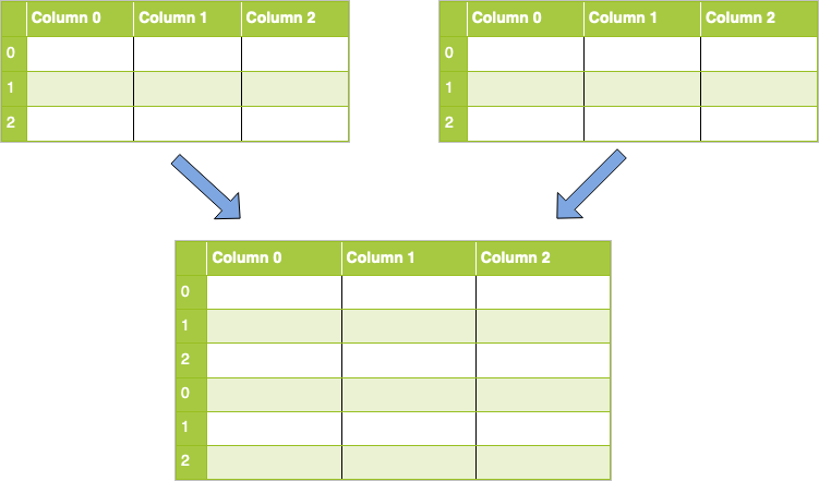
To implement this in code, you will use concat() and pass it a list of data frames that you want to combine. The code for this task will look like this:
concatenated = pandas.concat([df1, df2])
Note: In this example, it is assumed that the names of your columns match. If your column names are different when combining rows (axis 0), then by default the columns will also be added, and the values NaN will be filled in accordingly.
What if you want to join columns instead? First, take a look at the visual representation of this operation.:
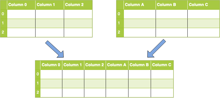
To achieve this, you will use the concat() call, as you did above, but you will also need to pass the axis parameter with the value 1 or "columns":
concatenated = pandas.concat([df1, df2], axis="columns")
Note: In this example, it is assumed that your indexes are the same for all datasets. If they differ when combined by column (axis 1), then additional indexes (rows) will also be added by default, and the values NaN will be filled in accordingly.
You will learn more about the parameters for concat() in the section below.
How to use concat()
As you can see, concatenation is an easier way to combine datasets. It is often used to form a single large data set with which additional operations can be performed.
Note: When you call concat(), a copy of all the data that you combine is created. You should be careful with multiple calls concat(), as a large number of running copies can negatively affect performance. Alternatively, you can set an optional parameter copy to False
When combining data sets, you can specify the axis along which the merging will be performed. But what happens to the other axis?
Nothing. By default, merging results in an installed merge, in which all data is saved. You've seen this with merge() and .join() as an external connection, and you can specify this using the parameter join.
If you use this option, the default value is outer, but you also have the option inner, which will perform an internal connection, or set the intersection.
As with the other internal connections you've seen before, there may be some data loss when making an internal connection using concat(). Rows or columns are saved only if the axis labels match.
Note: Remember that the join parameter only determines how to handle the axes that you do not combine along.
Since you have learned about the join parameter, here are some other parameters that accepts concat():
-
objsaccepts any sequence — usually a list — ofSeriesorDataFrameobjects to be combined. You can also provide dictionary. In this case, the keys will be used to build a hierarchical index. -
axisit represents the axis along which you will connect. The default value is0, which is combined by index, or row axis. Alternatively, the value1will be combined vertically, along the columns. You can also use string values"index"or"columns". -
joinit is similar to thehowparameter in other methods, but it takes only the valuesinnerorouter. The default value isouter, which preserves the data, whileinnerexcludes data that does not match in another dataset. -
ignore_indextakes the boolean valueTrueorFalse. The default value isFalse. IfTrue, the new combined dataset will not preserve the original index values on the axis specified in theaxisparameter. This allows you to get completely new index values. -
keysallows you to create a hierarchical index. One common use case is to create a new index while preserving the original indexes so that you can identify which rows, for example, are taken from which original dataset. -
copyspecifies whether you want to copy the source data. The default value isTrue. If the valueFalseis set, pandas will not create copies of the source data..
This list is not exhaustive. You can find a complete and up-to-date list of parameters in the pandas documentation..
Examples
First, you'll perform basic concatenation on the default axis using the data frames you've been playing with throughout this tutorial.:
>>> double_precip = pd.concat([precip_one_station, precip_one_station])
>>> double_precip.shape
(730, 29)
This file is very simple in design. Here you have created a data frame that is a duplicate of the small data frame you created earlier. It should be noted that the indexes are repeated. If you need a new index based on 0, then you can use the parameter ignore_index:
>>> reindexed = pd.concat(
...     [precip_one_station, precip_one_station], ignore_index=True
... )
>>> reindexed.index
RangeIndex(start=0, stop=730, step=1)
As noted earlier, if you combine data on the 0 axis (rows), but the labels on the 1 axis (columns) do not match, then these columns will be added and filled with values NaN. This results in an external connection:
>>> outer_joined = pd.concat([climate_precip, climate_temp])
>>> outer_joined.shape
(278130, 47)
In these two data frames, because you're just combining rows, very few columns have the same names. This means that you will see many columns with values. NaN.
To delete columns that lack any data instead, use the join parameter with the value "inner" to perform an internal join.:
>>> inner_joined = pd.concat([climate_temp, climate_precip], join="inner")
>>> inner_joined.shape
(278130, 3)
When using an internal join, you will only have those columns that are common to the original data frames.: STATION, STATION_NAME, and DATE.
You can also change this by setting the parameter axis:
>>> inner_joined_cols = pd.concat(
...     [climate_temp, climate_precip], axis="columns", join="inner"
... )
>>> inner_joined_cols.shape
(127020, 50)
Now you have only those rows that contain data for all columns in both data frames. It is no coincidence that the number of rows corresponds to the number of rows in a smaller data frame.
Another useful technique for combining is to use the keys parameter to create hierarchical axis labels. This is useful if you want to keep indexes or column names of the original datasets, but also want to add new ones:
>>> hierarchical_keys = pd.concat(
...     [climate_temp, climate_precip], keys=["temp", "precip"]
... )
>>> hierarchical_keys.index
MultiIndex([(  'temp',      0),
            (  'temp',      1),
            ...
            ('precip', 151108),
            ('precip', 151109)],
           length=278130)
If you check the original data frames, you can check whether the higher-level axis labels temp and precip have been added to the corresponding lines.
Conclusion
Now you have learned the three most important methods of combining data in pandas:
merge()to combine data by common columns or indexes.join()to combine data into a key column or indexconcat()to combine data frames by rows or columns
In addition to learning how to use these techniques, you also learned about set logic by experimenting with different ways to combine your datasets. In addition, you have learned about the most common parameters of each of the above methods and what arguments you can pass to customize their output.
You have seen these methods in action on a real dataset obtained from NOAA, which has shown you not only how to combine your data, but also the benefits of using the built-in pandas methods. If you haven't downloaded the project files yet, you can get them here:
Download the notebook and data set: Click here to get the Jupyter notebook and the CSV dataset that you will use to familiarize yourself with Pandas, this guide uses the merge(), .join() and concat functions.().
Back to Top